ALGOSAVE was mentioned in the news

https://www.risk.net/our-take/6288486/credit-risk-quants-are-hitting-tech-gap

ALGOSAVE is proud to join RBS Natwest FinTech Accelerator

Gordon Merrylees, Managing Director Entrepreneurship, NatWest said “We are delighted to welcome David Botbol and ALGOSAVE on to the programme in London. ‘With our unique offering that provides the right environment, coaching and networks, we help entrepreneurs start, scale and succeed every day.” We look forward to seeing David engage with the programme and grow ALGOSAVE business with us.”

ALGOSAVE offers to bond – and credit – investors high-yielding and risk-return efficient bond issues and credit portfolios. Bundled with peace of mind and BANG ON their risk-return TARGET.

ALGOSAVE offers to bond – and credit – investors its proprietary selection of the most high-yielding and risk-return efficient bond issuers and credit portfolios.
Directly from ALGOSAVE proprietary issuer database, bundled with peace of mind and BANG ON investors risk-return target.

ALGOSAVE carefully – and fully automated – selected credit portfolios are based on ALGOSAVE proprietary FINancial TECHnology which leverages three innovative concepts, borrowed from the banking industry :

1. Bond issuer Expected Credit Loss & Expected Return : ALGOSAVE proprietary financial technology selects the most risk-return efficient corporate bond issuers using their respective Expected Credit Loss & their respective Expected-Return term structure. ALGOSAVE ECL handily merges 2 credit-specific risk metrics : Probability and Default (PD) and Loss Given Default (LGD) term structure.
   Issuers must also first pass thru ALGOSAVE proprietary stringent selection process which protects investors while also allowing them to reach out for high-yielding assets with greater peace of mind. For instance, even a “CCC+” rated 5-year corporate bond – with its 11% credit spread above risk free rate – also appears on ALGOSAVE issuer radar screen.
2. Portfolio Expected Loss : ALGOSAVE proprietary FINancial TECHnology builds risk/return efficient high-yielding bond portfolios using the Expected Loss concept. The EL is instrumental in (a) creating investor specific and optimal risk-return asset allocation as well as (b) nourishing an informed dialogue between investors and their investment/financial advisers.
3. Putting issuers and portfolios thru ALGOSAVE proprietary stress-testing technology, ALGOSAVE offers high-yielding, diversified and risk-return efficient bond portfolios for investors with high, average and low risk appetite.

1 – Background.

Many tools and platforms have been developed to build efficient financial assets portfolios.
Those traditional tools are founded on some variation of Nobel prize winning Markowitz efficient frontier which selects asset portfolio based on their risk/return profile : the famous Efficient Frontier.

However, and in addition to typical Markowitz volatility of portfolio return, bond-portfolio investments are also sensitive to their asset-class specific risks : (1) a credit downgrade and  (2) a full-blown bankruptcy.

a – The first one – a credit downgrade – may force bond investors to sell.
Indeed, should a bond issuer credit rating move beyond their investment constraints (e.g high grade only) they will have to sell its bond and reinvest their proceeds – at a loss – into an investment policy compliant bond. This risk of downgrade is directly – and usually ahead of time – reflected in the bond-issuer Probability of Default term structure (PD)

b –  The second one – a full blown bankruptcy – will force bond investors to “go to” recovery together with the other stakeholders with equal seniority ranking. The loss here is BIG. It is best measured by issuer and seniority specific Loss Given Default term structure (LGD)

Some attempts to tackle these missing bond-specific risk metrics have been made where credit quality proxies such as credit rating or/and typical leverage ratio – NetDebt/Ebitda or FFO/NetDebt – are used as run-of-the-mill measures for credit and bankruptcy risk.

Unfortunately those proxies are not completely helpful : they are not easily translated into quantifiable risk-measures which in turn can be used in a risk-return bond selection and bond portfolio building.

2  – ALGOSAVE mission : bridge that gap and empower bond investors with a simple, turn-key and efficient bond-portfolio building platform.

Borrowing from BASEL banking regulation framework  – ALGOSAVE team is full of former bankers, so it is OK -, ALGOSAVE introduces bond-issuer specific Expected Credit Loss (ECL), and its portfolio-wide equivalent the Expected Loss (EL), as natural candidates for bond and bond portfolio tailor-made risk metrics.

First, let’s define each of them :
a – Expected Credit Loss = Loss Given Default x Probability of Default x Exposure At Default = LGD x PD x EAD
b – Expected Loss = the maximum bond portfolio loss with a chosen degree of confidence.

Nice things about ECL and EL ? Unlike rating or financial ratios, they are easily quantifiable and therefore, they can naturally be used to :
– (1) select risk-return efficient bonds and,
– (2) build risk-return efficient bond portfolio.

Indeed, the ECL merges together quantifiable PD and LGD term structure. This means that it can naturally be used as palatable single bond risk-metric.
In turn, the EL is a powerful tool for 2 reasons :
(a) ALGOSAVE EL in instrumental in creating investor specific and optimal risk-return asset allocation. Indeed, it directly determines the exact quantity of bonds to create optimal diversified portfolio by simply measuring bond portfolio diversification effect. The rest could be invested into other asset classes.
(b) By providing the maximum portfolio loss with a given degree of confidence (95%, 99% and even 99.9%) ALGOSAVE EL nourishes an informed dialogue between investors and their assets managers.

3.  Now that we have selected the right bond-specific risk metric, let’s build efficient bond portfolios with ALGOSAVE bond platform.

Now that investors have selected those precious bonds and bond-portfolio specific risk measures (respectively ECL and EL), let’s allocate investors’ hard earned moneys using those metrics.

First Step : Unlike share investors, beside pocketing their bond’s Yield To Maturity (YTM), bond investors enjoy little other upside. After all, as 1997 Nobel Prize Robert C. Merton showed it, bond investors are selling to shareholders a put option on the value of the assets of the bond issuer. Their maximum return is therefore the put option “premium” – a.k.a. the Bond Yield To Maturity – while their downside is unlimited – they can lose 100% of their investment. Doesn’t this requires extra care ?

4. This is why – at ALGOSAVE – bond issuers must go thru tough filters in order to become eligible for investors.

Every bond issuer first goes thru Algosave proprietary scoring technology which selects only those issuers where debt capital valuation and equity capital valuation simultaneously tell the same story. They must also adequately reflect the current risk profile of the corporate. The latter takes into account sales growth – with its past volatility and future sustainability – cash flow generation capacity – with its predictability and stability – operating and financial leverage – with their predictability and model-ability and many more risk parameters.

5. ALGOSAVE tough selection protects investors while also allowing them to reach out for high-yielding bonds with greater peace of mind.

Let’s start by selecting those bonds which will give investors the largest amount of yield per unit of risk. What we call the most efficient bonds.

To achieve this, ALGOSAVE computes the following ratio – also know as Sharpe Ratio – [Expected Bond return – Risk Free Rate] / Expected Bond Risk.

This graphs depicts a selection of 6 bond issuers from ALGOSAVE list of the 22 best risk/return 5-year maturity bonds (from ALGOSAVE bond platform) . The “22” will be explained later on. To the best of our knowledge, it has nothing to do with a “catch 22” 🙂

6. Now that we have sorted those bonds according to their risk-return efficiency, which, and how many bonds do we put in our 5-year portfolio ?

With ALGOSAVE bond platform, answering those 2 questions is simple and straightforward.

Which bonds come into our portfolio ?
We will build our proposed 5-year maturity portfolio by selecting those Sharpe ratio sorted bonds starting form the most efficient bond and going down the list.

How many bonds ?
The objective is to find the optimal number of bonds where the portfolio diversification effect is at its best. This graph shows that this optimal point resides on bond number 22. Of course, this all has to do issuer Probability of Default and LGD as well as with their correlation term structure (PD, LGD and PD-LGD correlation). We have written a few lines about these in those posts here, here, here,  and here.

The y-axis of the here-under  graph shows the expected credit loss within 5 years expressed in percentage of the initial investment with a portfolio of 1,2,3….123 bonds.

7 – ALGOSAVE proposed portfolio expected return above risk-free rate stands at 6.77% over the next 5 years.

For comparison sake, This is more than double the expected return above risk free rate on a portfolio of US banks over the same period

Let’s first examine the Expected Return of the equally weighted portfolio of those here-above 5-year maturity bonds. For each issuer, the expected return is computed as the survival rate weighted-average of its 5-year YTM. For instance when the 1-year PD = 1%, the survival rate is 99%, and the expected return becomes : Bond YTM x 99%.

As shown in the here-under sample table, the portfolio Expected Return above risk free rate – which is the is average of its constituent bonds Expected Return – is 6.77% over the next 5 years which is, for instance, more than double the expected return above risk free rate on a portfolio of US banks.

8 – From an efficiency point of view, the proposed 5-year portfolio is BANG on target.

The proposed 5-year portfolio is BANG on target. Indeed the portfolio 6.77% Expected Return exactly compensates the portfolio 6.78% Expected Credit Loss at the 99.9% confidence interval. This gives a Sharpe Ratio of 1.

Finally, ALGOSAVE palatable bond portfolio Expected Loss metric is far better suited to measure bond-portfolio Loss – at 50%, 95%, 99% or 99,9% even confidence interval – than credit rating, return volatility or any financial ratio for the matter.

Hence, the portfolio average (expected) credit loss for OECD consensus macro scenario and for ALGOSAVE stress-tested macro scenario are respectively 0.37% and 1.09%. The portfolio maximum losses (at 95% and 99% confidence interval) are respectively 2.66% and 4.27% (in OECD  consensus macro scenario) and 5.38% and 9.08% (in ALGOSAVE stress-tested macro scenario).

Conclusion : by mixing together issuer specific credit risk metrics (PD and LGD) as well as their scenario sensitive correlation term-structure , ALGOSAVE bond platform empowers bond-investors with a simple high-yielding and risk-return efficient bond-portfolio building platform. Bundled with peace of mind.

Of course, real-life bond portfolio must be tailor-made to investors risk and return objectives, time horizon, liquidity, tax, legal and unique circumstances.

For a complete list of ALGOSAVE most efficient corporate bond issuers as well as for ALGOSAVE risk-averse and risk-hungry credit portfolios, fill in the following form and send it ! We will graciously send them to you.

 

Name(required)

Email(required)

Website

Message

Submit

Δ

45% lower Economic Capital requirement on a typical corporate loan portfolio ? YES, it is possible with ALGOSAVE. And not just during the Tour de France.

45% lower economic capital requirements on a typical corporate loan portfolio ? yes it is possible with ALGOSAVE proprietary financial technology. And not just during the Tour de France.

45% lower economic capital requirements on a typical corporate loan portfolio ? yes it is possible with ALGOSAVE Financial Technology combination of
– borrower & seniority specific Loss Given Default (LGD) term-structure, and
– deep financial-analysis driven Default Probability (PD) and Joint-PD correlation term-structure.

Background :

The main drivers of Economic Capital estimates are :
– Loss Given Default (LGD),
– default probability (PD),
– and at a credit portfolio level, Joint PD correlation.

Let’s review each of those critical component with ALGOSAVE proprietary Financial Technology and see why and how ALGOSAVE helps banks save substantial capital.

1 – Seniority specific and economic-cycle sensitive Point in Time Loss Given Default (LGD) term structure:

ALGOSAVE addresses the 2 main drawbacks of traditional LGD “Beta” distribution model :
– uni-modality : where empirical evidence show that recoveries are – at least – bi-modal, with typical peaks at 20% and 80%
– difficulty to cope with “point masses” at 0% and 100%, where empirical evidence also show that LGD are often located in those areas.

Simple solution : ALGOSAVE financial technology GOT RID of LGD Beta model.

ALGOSAVE proprietary Financial Technology (FinTech) projects corporate financial statements – 100 data points – using Montecarlo simulations. This allows ALGOSAVE FinTech to reflect each corporate specific asset and leverage structure in each of its thousands of Montecarlo simulations paths at 3 different level of seniority : secured, unsecured and subordinated.

For instance, let’s assume that on a given path of its Montecarlo projections, McDonald (MCD) net debt is greater than its Enterprise Value in year 1. This comes – for instance – from higher capital expenditure than average. Assuming that, at the same time, MCD must draw on its Revolver Credit Facility – for instance to fund a greater than optimal sales growth rate – ALGOSAVE Financial Technology “pushes” MCD in default on that specific path.

ALGOSAVE then computes recovery using MCD specific debt and MCD specific asset liquidation value upon default . The latter takes into account 2 possible Machine Learning based outcomes : (1) a gone concern liquidation value, where MCD is taken over (at a multiple of sales or EBITDA) and keeps operating – or (2) a fire sale of MCD assets which price depends on the then Machine Learning Based economic cycle.

Following this methodology, this graph depicts the unsecured 1-year LGD distribution of a typical portfolio of 100 corporates selected from ALGOSAVE issuer database. And not Singapore skyline. The x-axis measures the LGD between 0 and 1.0 while the y-axis measures the number of observations of each bar in the histogram

First observation ? Both the multi-tail and “point mass” nature of ALGOSAVE proprietary LGD distribution clearly shine.

The blue LGD histogram depicts the LGD distribution for OECD consensus growth scenario with 59% average LGD – close to Basel Foundation 55% LGD and CDS 60% standard ISDA LGD. Examining the red histogram – which depicts the LGD distribution for ALGOSAVE stressed macro economic scenario – it is interesting to notice the marked shift of the LGD distribution from left (15% “blue” LGD) to right (100% “red” LGD). The average ALGOSAVE stressed-scenario LGD stands at 72%.

2 – Point in Time Probability of Default term structure :

ALGOSAVE Probability of Default (PD) term structure is calibrated on capital market PD term structure which comes from CDS, bonds and/or secondary loan trading.
It can also be calibrated on ALGOSAVE clients’ internal Point-in-Time default probability term structure.

This calibration gives ALGOSAVE PD term structure its unique “live” flavor which – by the way – is required by new accounting regulations.

3 – Joint PROBABILITY OF DEFAULT correlation :

ALGOSAVE proprietary joint PD correlation technology is a lot lower than its ill-fated CDS and equiy price correlation proxies. Those are full of “market noise” such as iTraxx CDS sector and ETF trading and hide real default correlation.

But, CLO traders and loan/bond portfolio managers are well aware of this phenomenon whereby actual default correlation – to the exception of those in the highly regulated financial sector – is a lot lower than its capital market proxies.

You may be interested by one of our latest posts which dealt with this issue in greater detail. Read it all here.

Conclusion – ALGOSAVE proprietary Financial Technology helps banks save 45% in economic capital

Indeed, putting all things together – LGD, PD and Joint PD correlation – where traditional Expected Loss model points toward a 3.30% Economic Capital requirement (on the sample corporate portfolio), ALGOSAVE proprietary Financial Technology only requires 1.80% Economic Capital at 99.9% confidence level.

A 45% saving on Economic Capital !

Now, that’s something worth celebrating. And, not just among our Welsh Tour de France cycling fans 🙂

Make your V.I.P. corporate client happy with TAILOR MADE COVENANTS, while watching out for COVENANT BUSTERS : meet ALGOSAVE unique PROBABILITY OF BREACH OF COVENANT.

Thanks to ALGOSAVE unique PROBABILITY OF BREACH OF COVENANT, it is now EASY to : 

• Make V.I.P. corporate clients happy by giving them greater financial flexibility thru tailor-made financial covenants.
• While, at the same time (since breaching a covenant means an IFRS9-related immediate hit to Net Income) watch out for potential covenant busters.

1 – Make V.I.P. corporate clients happy by giving them greater financial flexibility thru tailor-made financial covenants.

For instance, what if you could Increase your VIP corporate client financial flexibility – and even profitability – by granting them a 3.6 NetDebt-to-Ebitda covenant instead of an “automatic” 3.5 times ?

• First good piece of news : by doing this you help your VIP corporate client increase its financial flexibility and debt capacity.
  This means a lot to its CEO  : more M&A, more Capex, more working capital…
• Second good piece of news : you can also announce your VIP client that this means an $ XYZ additional  Return On Invested Capital – ROIC.
  This also means a lot and to a lot of people, starting – of course – with your VIP client’s shareholders.
• Third REAL good piece of news : you have probably won the origination / underwriting contest, by making a REAL difference…
  And, this means a lot to YOU.

What does it mean from the bank’s perspective, for instance on a 2-year Revolver Credit Facility ?

Meet ALGOSAVE unique Probability of Breach of Covenant.

For instance, and in ALGOSAVE benign macro economic scenario, ALGOSAVE PROBABILITY OF BREACH OF COVENANT shows that, giving this additional leeway to BP PLC means that the Bank keeps 87% of the quality of its early warning bankruptcy protection.

Indeed, the probability of breaching the x3.5 NetDebt to EBITDA covenant stands at 8.09% and drops to 7.01% (a 13% drop) at x3.6. The Bank will “miss” 13% of the total covenant breaching events when granting a x3.6 instead of a x3.5 turn of leverage covenant.

In ALGOSAVE stressed macro economic scenario,  the Bank keeps 93% of the quality of its early warning bankruptcy protection.

This marked difference in probability of breach of covenant is not found in the case of Exxon. In both case, the quality of the bank bankruptcy hedge is kept at 96%.

Hence although granting a 3.6 leverage covenant – instead of a 3.5 leverage – to BP PLC. might be questionable, it is a “no brainer” in the case of Exxon Mobil.

2. Beside gaining a competitive edge, knowing the probability of breaching covenant becomes critical to the P&L of IFRS-reporting Financial Institutions.

 

• Indeed, under IFRS9 rules, a breach of covenant triggers an immediate move from 12-month ECL – Stage1 – to lifetime ECL – Stage2.
• This means a significant increase in Expected Credit Loss with its immediate hit to P&L.
• As illustrated in the here-above table, behind the “one-size-fit-all” x3.5 NetDebt-to-EBITDA covenant, hides a broad range of probability of breaching this covenant within the next 2 years : from Statoil 3.18% to BP. PLC 36.42% goinf thru Royal Dutch Shell 13.51%.
• Below the quiet and reassuring surface of  traditional “one-size-fit-all” covenants, hides a boiling reality : degrees of operating and financial leverage, free cash flow volatility, sensitivity to macro economic scenario – and many other parameters – explain this diversity.
• Endowed with ALGOSAVE probability of Breach of Covenant, credit and risk management committees build a watch list of possible covenant busters. This simple – yet powerful – tool guides them to take action before a sudden breach of covenant immediately hits P&L. They have seen it coming.

Ask for your private access to ALGOSAVE CORPORATE UNDERWRITING PLATFORM, and see how you can SECURE UNIQUE COMPETITIVE edge with your VIP clients while BEING ON THE WATCH for possible COVENANT BUSTERS.

Name(required)

Email(required)

Website

Message

Submit

Δ

The missing link : PD-LGD correlation – almost – holds true throughout the term structure of forward looking Point-in-Time PDs and LGDs

There is empirical evidence of high Default – Loss Given Default correlation. This historical phenomenon is also known as high PD-LGD correlation.
Indeed, historically and during periods where there is a relatively high number of corporate defaults, the average Loss Given Default – LGD – is also relatively high. And, the opposite is also true. During periods where there are relatively few default occurrence, LGDs are relatively low on those occurrences.

Does this empirical observation also hold true throughout the term structure of forward-looking and Point-in-Time PDs and LGDs ?

ALGOSAVE new valuation paradigm confirms that PD-LGD correlation – almost – holds true throughout the term structure of forward-looking & Point-in-Time PDs and LGDs.

Contradicting this intuitive correlation, there are also cases whereby benign macro-economic LGDs are as high or even greater than stressed LGDs. This phenomenon mostly happens towards the end of the term structure.

We will illustrate this finding with a few examples that all come from ALGOSAVE CORPORATE ISSUER DATABASE.

For instance here are ALGOSAVE unsecured 3-year,5-year and 10-year LGD distributions for 3 Integrated Oil and Gas companies : BP PLC., Occidental Petroleum and Royal Dutch Shell.

The blue bars in the histogram illustrate the LGD distribution in benign – consensus – macro economic scenario, while the red bars depict the LGD distribution in ALGOSAVE stressed macro-economic scenario. The first, second and third histograms – from top to bottom – respectively depict the distribution of the 3-year, 5-year and 10-year unsecured LGD.

For instance, in the case of BP PLC – the first histogram at the top – whereas the consensus 3-year unsecured LGD (in blue) are distributed between 40% and 63%, the stressed LGDs (in red) are distributed between 73% and 98%. As shown in the other 2 histograms, this marked difference between ALGOSAVE 2 LGD regimes (benign and stressed) also holds true both for the other 2 corporates at the 3-year point. Although there is already a little overlap for Occidental Petroleum.

This PD-LGD correlation almost holds true throughout the scenario-sensitive LGD term structure. Indeed, from 3-year to 10-year, the LGD of ALGOSAVE benign economic scenario – associated to lower PDs – are generally lower than those of ALGOSAVE stressed scenarios – associated with higher PDs.

However, those 2 LGDs regime sometime overlap. This is the case of BP PLC and Royal Dutch Shell 10-year LGD distributions, where the blue bars (benign scenario) overlap with the red bars (stressed scenario)

Validating empirical findings, ALGOSAVE confirms that PD and LGD are correlated throughout the term structure albeit with some overlap.

Those LGD term structure are delivered by ALGOSAVE ISSUER DATABASE and are directly related to the the here-under ALGOSAVE scenario-sensitive PD term structure and EV distribution :

• Forward looking, scenario-sensitive Default Probability Term Structure  : consensus (in blue), very good macro economic scenario (in green), stressed macro economic scenario (in red) for BP PLC., Occidental Petroleum and Royal Dutch Shell
• Consensus (in blue) and stressed (in red) Asset Value (EV) distributions for BP PLC., Occidental Petroleum and Royal Dutch Shell.

 

 

Good century-old DuPont-analysis helps Banks SAVE CAPITAL : what an explosive surprise !

 

Good century-old DuPont-analysis helps Banks SAVE CAPITAL : what an explosive surprise !

ALGOSAVE confirms DuPont analysis profound wisdom : LGD CORRELATION is ROCK-BOTTOM LOW and helps financial institutions SAVE CAPITAL.

And, especially for high grade borrowers, ALGOSAVE has another BIG surprise in store on PD-LGD correlations.

DuPont Analysis comes from the DuPont Corporation that started using this formula in the 1920s.
DuPont explosives salesman Donaldson Brown invented this formula in an internal efficiency report in 1912.

More than a century after that, ALGOSAVE CORPORATE DATABASE shows that DuPont analysis also hides another even more profound wisdom : the CORRELATION of Loss Given Default (LGD) between corporates in a given industry is ROCK BOTTOM LOW to negative. This means IMMEDIATE CAPITAL SAVING for corporate lenders.

In The Beginning, long time ago.

DuPont analysis tells us that the Return On Equity – ROE – can be decomposed in 3 items

Net Income / Sales = Profitability
Sales / Total Assets = Asset Efficiency
Total Assets / Average Shareholder Equity = Financial Leverage

1. DuPont analysis also tells us that profitability is mostly matter of technology.
   In other word, when a company is part of a given industry, it “inherits” the industry profitability which is technology-dependent.
   For instance, if you distribute food in the US, your expected Net Income / Sales cannot be too-far away from your peers. Unless you have a completely different service or…technology.
2. DuPont analysis also tells us that Asset Efficiency is mostly a matter of the corporate competitive landscape.
   Indeed, in order to increase this ratio, the company will have to gain market share <=> increase marketing expenses, lower price, increase inventories to prepare for increased sales, and give longer credit to its clients <=> lower net Income and higher Total Assets.
   Profitability and Asset Efficiency are interdependent.
3. So, in order to increase its ROE and make a difference, the company’s management is mostly left with the latest ROE key driver : ITS degree of Financial Leverage. Let’s also keep in mind that an increase in financial leverage also means an increase in the Equity BETA, with its consequence on WACC and ultimately on the Expected ROE.

From DuPont analysis … to rock-bottom LOW LGD CORRELATION

If DuPont analysis holds true – and indeed corporates in the same industry mostly drive their ROE thru financial leverage – then when they go bankrupt together, we should be expecting little correlation between their respective Loss Given Default : they all finance their assets in a different way to make a difference in their respective ROE.

The challenge : historical high-grade corporates LGDs are scarce <=> Default of large and solid corporates are a rare event.
Concomitant defaults of such corporates are even rarer. So that measuring historical LGD correlation is a challenge.
Estimating forward looking and Point in Time LGD correlation is a double-challenge.

Algosave technology raises to the challenge and delivers its clients exactly that : forward looking and Point in Time stress-tested LGD correlations.
ALGOSAVE delivers those for all the 5000 borrowers in ALGOSAVE CORPORATE DATABASE.

Let’s take an example on our favorite Integrated Oil and Gas basket : 11 high-grade global corporates

ALGOSAVE CORPORATE DATABASE delivers the following data : average 5-year unsecured stressedLGD, current and stressed cumulative 5 year PD

1. Before the bigger surprise, let’s have a look at 5-year average stressed unsecured LGDs for each of those 11 corporates.Although the average LGD of those asset-heavy corporates is close to 49% – which is close to CDS standard LGD  – there is a marked difference between BP P.L.C. 81% 5-year LGD and Husky Energy 22% 5-year LGD.
   This already confirms DuPont analysis differing financial structure, albeit in a static and average way.
2. Let’s also compare current market 5-year PDs and ALGOSAVE stressed 5-year PDs.
   Although current 5-year cumulated PDs are multiplied by a factor of 5 when stressed (increase from 4% to 20%), BP and Statoil are multiplied by a factor of more than 10, whereas Husky Energy is only multiplied by a factor of 2.5.
   This also confirms DuPont analysis about differing financial structure, albeit in a static and average way.
3. Finally, last but not least, ALGOSAVE CORPORATE DATABASE unique and CAPITAL SAVING deliverable : Forward-looking, Point in Time and stressed 5 year unsecured LGD correlations
   
   On average stressed LGD correlation is a ROCK BOTTOM -0.01
   The highest LGD correlation is a small 0.11, between Royal Dutch Shell and EXXON.
   The lowest LGD correlation is also a small -0.13, between TOTAL SA and Suncor Energy.
   Thinking “DuPont”, this should not be surprising. Indeed, DuPont analysis implicitly states that in order to drive its ROE, company management is mostly left with carefully choosing its Degree of Financial Leverage. Hence is case of concomitant default of two corporates, lenders should not expect to loose the same amount of money on their debt.As a conclusion, ALGOSAVE confirms DuPont analysis profound wisdom : LGD CORRELATION is a ROCK-BOTTOM LOW and CAPITAL SAVING critical metric.
4. Last but not least ALGOSAVE ALSO offers a surprise on PD-LGD correlation in stressed scenario for high-grade borrowers.
   This will be the object our our next post. Please stay tuned.If you like this post, do not hesitate to ask for you free subscription :
   Name(required)

   Email(required)

   Website

   Message

   Submit

   Δ

ALGOSAVE elevator pitch with Mr. Jan Christopher Arp co-founder and Managing Partner @ Holt Fintech A.I Accelerator

Fintech Junction is one of the best organized FinTech event in Israel.

It comes bundled with interesting forums, attractive and engaged sponsors, as well as professionally organized 1-on-1 meetings opportunities.

One of those meeting gave me the opportunity to meet with Mr Jan Chritopher Arp, co-founder and Managing partner at Holt Accelerator – https://lnkd.in/e8t8B6n – which is one of the leading and most experienced family-office in the world.

Jan Christopher gave me the opportunity to make an ALGOSAVE elevator pitch : https://lnkd.in/egbMhPr

Thank very much Jan Christopher, and hopefully see you soon in Montreal ?

This time I will have a real opportunity to sing “Oh Canada, our home and native land, true patriot love in all of us command …” 😉

What is the WACC we – analysts – should be using to value a corporate Free Cash flow, and ultimately a corporate Enterprise Value – EV – ?

 

Since there is a credit spread curve, do we need a WACC curve, or can we resort to using one single WACC ?

Also, we all know that – theoretically – Equity BETA should be deleveraged and re leveraged as a function of corporate financial leverage dynamics. Should we be using one-single Equity BETA to compute the cost of Equity, or do we have to build a Beta Curve ?

Lets’s examine a few examples, to better measure and understand this twin challenge.

Here are the WACC distribution (the top image) and Equity BETA distribution (the bottom picture) for 4 major and global retailers : WALMART, THE KROGER, AHOLD and CARREFOUR.

• 1-year distribution in blue
• 5 year distribution in red
• 10-year distribution in green
  
• First observation : WALMART is unique : a relatively narrow bandwidth both in its BETA as well as in its WACC
• Second observation : in any case, what a world of difference between those corporates.
• Third observation : what a world of difference between between 1-year, 5-year and 10-year WACC and BETA distribution for every corporate.
• Final observation : even for a given year, what a broad distribution in the Equity BETA itself.

Can we answer the original question : for better issuer valuation, should we use a WACC and a BETA curve ? Probably so.

Ask for your private access to ALGOSAVE ISSUER DATABASE and check how you can increase the POWER AND UNIQUENESS of your financial analysis.

Name(required)

Email(required)

Website

Message

Submit

Δ

From Stress-Testing to Relaxing : what if banks could really SAVE CAPITAL ?

In stress-test scenarios, the assumption is : high correlation for everything.

We, bankers – and I used to be one – have been caught with our hand in the low correlation cookie jar. We decided to take action so that it won’t happen again.

To add to our comfort – or rather, discomfort really – markets are confirming our fears and react exactly this way . Looking at CDS prices one could even ask : why bother having one CDS per issuer ? Let’s just have one CDS per industry. One size fits all !

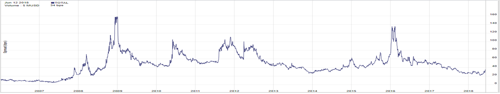
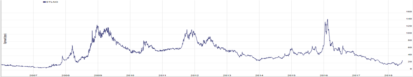
For example, the first CDS 5-year graph is that of Royal Dutch Shell (RDSA), the second one is that of Total SA, and the third one is that of Statoil (renamed Equinor).

Thanks to https://www.datagrapple.com/ for those graphs

Guessed the 85% correlation ?

Immediate consequence : in stress-test scenarios, banks must take into account this thru-the-roof – 85% – CDS implied Probability of Default correlation and put aside a lot of capital.

Why ? since defaults of rock-solid corporates – such as the one we just looked at – are very rate events, there are very little statistics of actual default contagion in high grade credit portfolios.

So, in order to measure default contagion, lenders are left using whatever proxy they can find. But, although CDS – or share, or bond – price correlation is the most obvious one, at 85% it is also a killer !

What if one could statistically measure this domino effect ? That is precisely what ALGOSAVE FinTech does. And it is definitively worth our while and that of our clients.

Indeed, ALGOSAVE shows that, even in very bad economic scenarios, default correlation is actually far lower than CDS thru-the-roof correlation suggests.

Here is an example on our favorite Integrated Oil and Gas portfolio.

For instance, whereas Total/RDSA 5-year CDS correlation is close to 85%, ALGOSAVE shows that it is actually closer to 25% even a very bad economic scenario. Arguably, it is still more that 3 times Total/RDSA conditional default probability in consensus OECD macro-economic scenario. But it is a far cry from the 85% CDS correlation mark.

Well done, from 85% down to 25% default correlation that’s tangible capital saving. It is well worth the time you just invested into reading this article till the end. And, should you want to see these default correlation for another industry, please leave us a comment here. We will graciously send this to you.

ALGOSAVE proprietary credit database is full of those precious nuggets … and some other too such as equity analyst favorite WACC and Beta. But, let’s leave these for our next article.

All the Best

ALGOSAVE team. 13th of June 2018.